Storage has changed more in the last two decades than many other parts of the computer. It has transitioned from mechanical hard drives with spinning platters rotating at thousands of revolutions per minute to flash memory-based units capable of handling thousands of operations in parallel with microsecond latencies. In practice, this evolution has not only accelerated boot times and application opening speeds: it has redefined database performance, virtualization, compilations, containers, and Artificial Intelligence workloads.
The clear consequence is this: choosing the wrong type of storage can turn a powerful server into a “slow” system in the user’s eyes, even if it has plenty of CPU and RAM. Doing it right, on the other hand, reduces latencies, improves productivity, and allows more services to be consolidated per node with fewer bottlenecks.
HDD: the veteran still indispensable (but not for everything)
A HDD (Hard Disk Drive) uses spinning magnetic disks and a mechanical head that moves to read or write data. This mechanical aspect introduces two unavoidable penalties: seek time (moving the head) and rotational latency (waiting for the sector to pass under the head). Therefore, while a modern HDD can offer reasonable sequential performance, it struggles especially with random access patterns.
Typically, a 7,200 rpm HDD moves around 80–160 MB/s in sustained sequential read/write speeds (depending on density and zone of the platter). The problem appears with random access: latency jumps to milliseconds, and IOPS (input/output operations per second) are well below any SSD.
Nevertheless, HDDs still hold a hard-to-beat value: cost per gigabyte. That’s why they remain the natural choice for:
- Mass storage (large files, multimedia, archives).
- Backups and “cold” repositories.
- Video surveillance and continuous recording (with units optimized for this load).
The technical recommendation is simple: HDD for capacity and retention; not for low latency or high-randomness environments (VMs, transactional databases, intensive logs).
SATA SSD: the ongoing transition still in production
SATA SSD eliminated the mechanical parts and replaced platters with NAND Flash memory. This alone drastically reduces latency and boosts perceived fluidity. However, these SSDs are still tied to an interface designed in the era of mechanical disks: SATA III (6 Gb/s), with a practical ceiling of about ~550 MB/s under real conditions.
The improvement over HDDs is compelling on two fronts:
- Latency: drops from milliseconds to microseconds.
- IOPS: significantly increases, especially for random reads.
Therefore, SATA SSDs remain a very solid option for:
- Revitalizing old equipment or servers without NVMe support.
- System volumes, boot drives, and general applications.
- Environments where access patterns do not demand extreme IOPS (e.g., moderate web services, internal tools, file servers with caching).
The real limit isn’t NAND technology itself; it’s the SATA “bottleneck” and its traditional stack (AHCI). This is a key technical point that explains much of the difference versus NVMe.
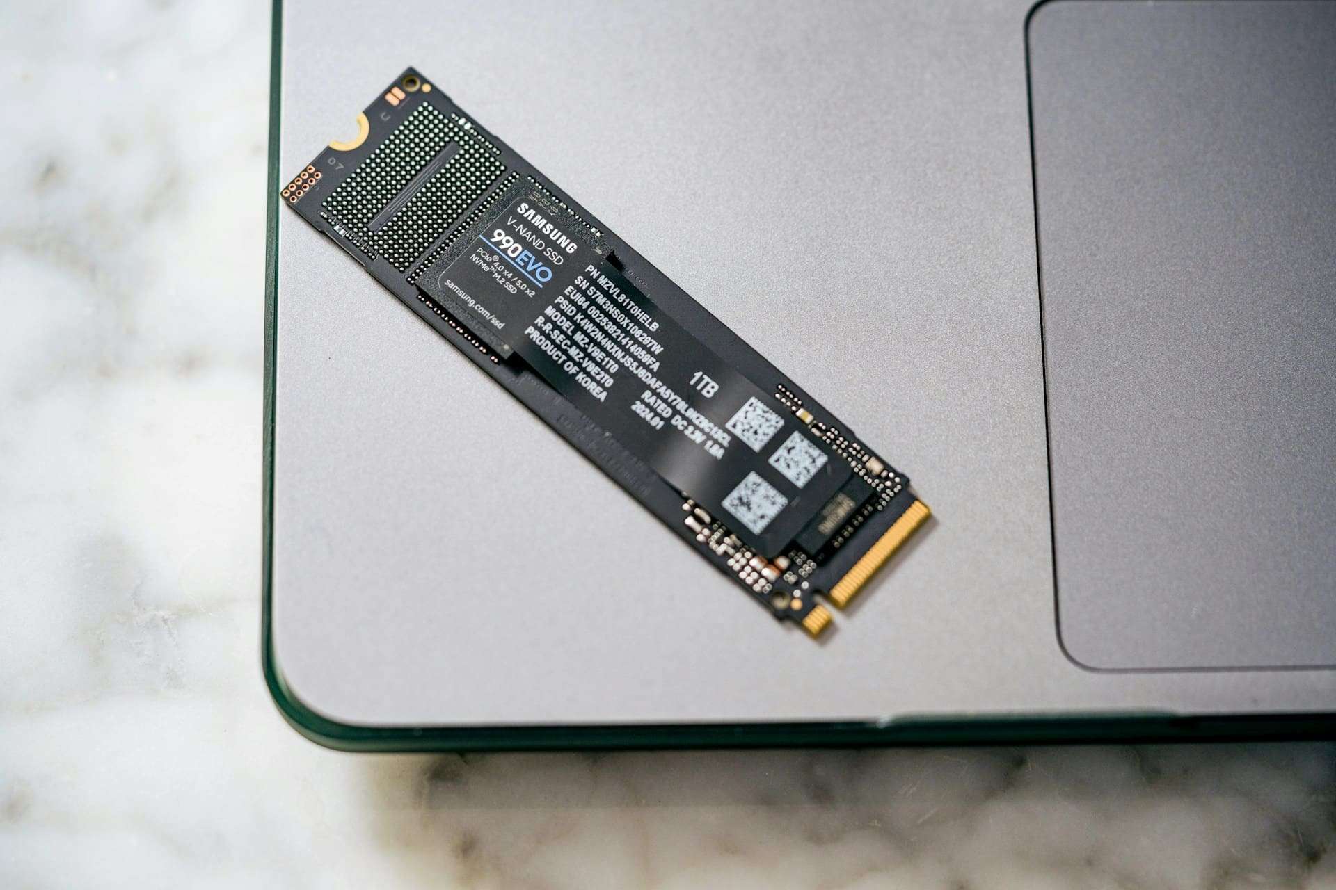
NVMe: when the bottleneck is no longer the bus
NVMe (Non-Volatile Memory Express) is not just “another SSD”: it’s a protocol specifically designed for flash memory that works over PCIe, exploiting modern hardware’s parallelism. While SATA/AHCI was built with mechanical disk assumptions, NVMe is born for deep queues, low latency, and massive concurrency.
In theoretical sequential speeds, typical market ranges (depending on generation, number of PCIe lanes, controller, and NAND) are as follows:
- PCIe 3.0: ~3,500 MB/s
- PCIe 4.0: ~7,000 MB/s
- PCIe 5.0: up to ~14,000 MB/s
But the most significant leap isn’t just in “MB/s”: it’s how NVMe manages simultaneous operations.
The queue depth difference that changes everything
- HDD and SATA SSD (AHCI): typically 1 queue with up to 32 commands.
- NVMe: up to 65,000 queues, with 65,000 commands per queue.
This architecture particularly impacts real multitasking: many small requests, high concurrency, multiple threads, containers, VMs, log queues, search indexes, database engines, and caches. In these scenarios, NVMe doesn’t just “go a little faster”: it fundamentally changes system behavior under load.
What marketing doesn’t always tell you: sequential speeds are not equivalent to real-world performance
Speeds of 7,000 or 14,000 MB/s are usually measured in ideal sequential scenarios. In real systems, performance is often dominated by 4K random I/O at low queue depths (QD1–QD4), where factors such as the following influence:
- Controller and firmware.
- NAND type and size (TLC/QLC) and SLC cache.
- Presence of DRAM in the unit (or HMB solutions in some models).
- Temperature and thermal throttling (especially in M.2 drives without proper cooling).
- File system and configuration (ext4, XFS, ZFS; alignment; TRIM/Discard).
Therefore, in professional environments, selection isn’t based solely on “MB/s” but on sustained IOPS, consistent performance under load, latency, and endurance.
How to choose: a quick guide by use cases
HDD
- Best for: backups, archiving, media, historical retention, video surveillance.
- Avoid for: operating systems, databases, intensive VMs, log queues.
SATA SSD
- Best for: servers and PCs needing clear improvement without changing platform; system volumes; moderate loads; general storage with good latency.
- Limitation: interface ceiling (~550 MB/s) and AHCI queue (32 commands).
NVMe
- Best for: virtualization with many VMs, databases, compilation and CI/CD, heavy video editing, analytics, fast cache storage, and AI pipelines where I/O feeds GPUs.
- Practical advice: ensure proper cooling, choose models with good sustained performance, and monitor endurance (TBW) if handling high write volumes.
Conclusion: the “disk” is no longer just a detail—it’s architecture
Today, storage decisions go beyond capacity. They depend on the latency the system responds with, the concurrency it can handle without degradation, and the performance ceiling when the server is fully loaded. HDDs, SATA SSDs, and NVMe don’t compete in the same arena: they are different tools for different problems. Aligning the type of unit with the load pattern (sequential vs. random, read vs. write, high vs. low concurrency) often yields improvements that even doubling the CPU cannot compensate for.
Frequently Asked Questions
What is the difference between speed (MB/s) and IOPS when choosing an SSD?
MB/s measures sustained transfer speed (ideal for large files). IOPS measure how many small operations can be done per second (critical for systems, databases, VMs, and containers). For perceived speed and real workloads, latency and IOPS often matter more.
Why might a SATA SSD feel fast but fall short in servers with many VMs?
Because SATA/AHCI operates with a single queue and up to 32 commands, limiting concurrency. Virtualization and databases have many simultaneous small requests; NVMe manages massive queues and reduces latency under load.
Is NVMe always better than SATA SSD for everything?
Not necessarily. For simple servers or older systems, a SATA SSD can offer a significant improvement at a lower cost. NVMe excels where there is high concurrency, random I/O, and heavy loads; in those cases, the differences are clear.
What should I watch out for when installing NVMe M.2 drives?
Temperature (can cause throttling), PCIe compatibility (generation and lanes), and sustained performance (not just peak speeds). For heavy write workloads, also consider endurance (TBW) and NAND type.